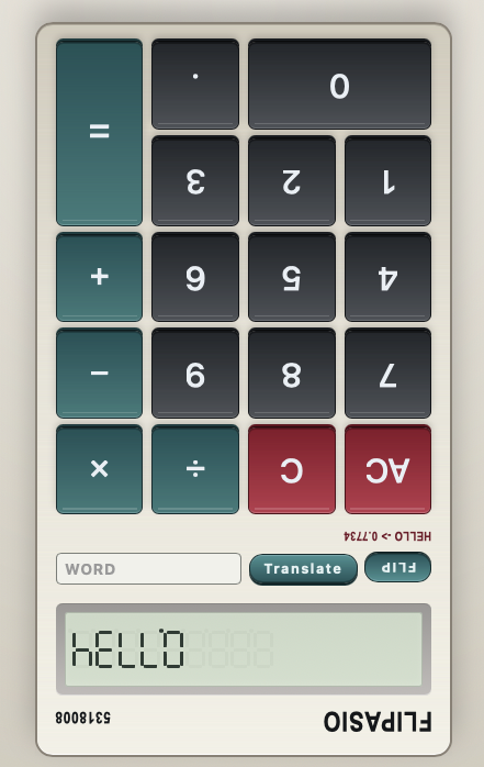
Categories
Best of Software Dev.

Classifying fruits with a Convolutional Neural Network in Keras

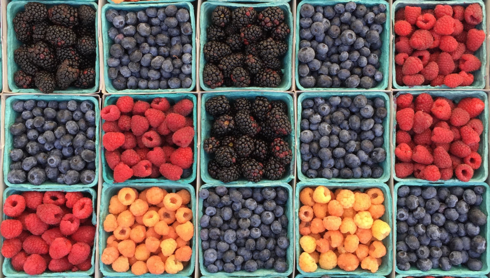
I followed a tutorial on Convolutional Neural Networks that left many questions unanswered. Soon I realized that the actual process of architecting a Neural Network and setting the parameters seemed to be much more experimental than I thought. It took a while to find explanations that a rookie like me could understand. Most of the posts I found gloss over the difficult details, like what NN configuration to choose, or which library to choose, or why would you use ReLU in an image-recognition NN  and focused on easier and more consistent tasks, like setting up a Python environment.


TL;DR

Keras allows you to build a neural network in about 10 minutes. You spend the remaining 20 hours training, testing, and tweaking.

If you wish to learn how a Convolutional Neural Network is used to classify images, this is a pretty good video.

The ultimate guide to convolutional neural networks honors its name.

This example illustrates how a CNN recognizes numbers: Basic Convnet for MNIST

Get the code at https://github.com/danielpradilla/python-keras-fruits.

Jump to the predictions.


A simple problem

In order to learn the basics, I started a simple —um, “simple”— project to build a deep neural network to correctly classify a set of 17 kinds of fruits from the Kaggle Fruits 360 dataset.

Keras provides an easy interface to create and train Neural Networks, hiding most of the tedious details and allowing you to focus on the NN structure. It interfaces with the most popular NN frameworks: Tensorflow, CNTK, and Theano. This answered one of my first questions, “Keras vs Tensorflow, which one should you learn and when to use each one?” —short answer: learn Keras until you need Tensorflow.

Keras allows you to go from idea to working NN in about 10 minutes. Which is impressive. The Keras workflow looks like this:

  • Get training and testing data
  • Define the layers
  • Compile the model
  • Train model
  • Evaluate the model
  • Get predictions

Get training and testing data

Keras provides a neat file-system-based helper for ingesting the training and testing datasets. You create a “training” and “validation” folder, and put your images there. In the case of a multi-category classifier like this one, each image class will have their own folder —”Apple”, “Oranges”, etc. flow_from_directory() will automatically infer the labels from the directory structure of the folders containing images. Every subfolder inside the training-folder (or validation-folder) will be considered a target class.

Alternatively, you can ingest the data on your own and do a manual split.

flow_from_directory is a property of ImageDataGenerator, a generator class that offers a memory-efficient iterator object. When you have large datasets it’s always wise to use a generator that yields batches of training data. More info at “A thing you should know about Keras if you plan to train a deep learning model on a large dataset

Remember that, even though we clearly see that this is an avocado, all the neural network may see is the result of some edge-detection filters. So an avocado is this apparently green oval thing placed in the middle of the field. If you train the NN with perfectly-centered avocados and then feed it an off-center avocado, you might get a poor prediction.

In order to account for this and facilitate the training process, Keras provides the ImageGenerator class, which allows you to define configuration parameters for augmenting the data by applying random changes in brightness, rotation, zoom, and skewing. This is a way to artificially expand the data set and increase the robustness of the training data.

One particularly important image augmentation step is to rescale the RGB values in the image to be within the [0,1] range, dividing each color value by 255. This normalizes the differences in pixel ranges across all images, and contributes to creating a network that learns the most essential features of each fruit. More info at Image Augmentation for Deep Learning with Keras.

test_gen = k.preprocessing.image.ImageDataGenerator(
rotation_range=0.1,
width_shift_range=0.1,
height_shift_range=0.1,
brightness_range=[0.5, 1.5],
channel_shift_range=0.05,
rescale=1./255
)

test_images_iter = test_gen.flow_from_directory(TEST_PATH,
target_size = TARGET_SIZE,
classes = VALID_FRUITS,
class_mode = 'categorical',
seed = SEED)

More image training data

There are a couple of datasets that are commonly used for training Neural Networks
COCO
CFAR

Network Architecture

What is the configuration of the Neural Network? How many convolutional layers, how many filters in each convolutional layer and what’s the size of these filters? These were some of the questions that arose as I started to read tutorials, papers, and documentation. Turns out that in the majority of the cases, the answer is “it depends”. It depends on the data, your previous decisions on image size, your goals in terms of accuracy/speed, and your personal understanding of what you deem a good solution.

Understanding Convolutional Neural Networks

This guide presents a high-level overview of the typical neural network structures that you can build in Keras: https://keras.io/getting-started/sequential-model-guide/

I watched a bunch of videos and this one provides the best explanation of what is a CNN and how it works:

The ultimate guide to convolutional neural networks honors its name. But the best way to understand how a CNN and each layer works at the most fundamental level is with these two examples:

Basic Convnet for MNIST

The number game

Layers are the building blocks of Neural Networks, you can think of them as processing units that are stacked (or… um… layered) and connected. In the case of feed-forward networks, like CNNs, the layers are connected sequentially. Commonly, each layer is comprised of nodes, or “neurons”, which perform individual calculations, but I rather think of layers as computation stages, because it’s not always clear that each layer contains neurons.

The process of creating layers with Keras is pretty straightforward. Just call keras.layers and push them into a list.

The two questions I found the hardest to answer were How many layers do I have to set up? and What is the number of nodes in each one? These are often overlooked in tutorials because you are just following the decisions of someone else. I bet that in the coming months we will see an abstraction similar to Keras with which you won’t even have to think of the number of layers.

The easy layers to figure out are the input and output layers. The input layer has one input node and in Keras there is not need to define it. The output layer depends on the type of neural network. If it’s a regressor or a binary classifier, then it has one output —you are either returning a number or a true/false value. If it’s a multi-class classifier with a softmax function at the end, you will need one node per class —in our case, one per type of fruit we are attempting to classify.

rtn = k.Sequential() #input

##something??

rtn.add(k.layers.Dense(units = len(trained_classes))) #output

Now, for the hidden layers, we need to think about the structure of a Convolutional Neural Network. In general terms, Convolutional Neural Networks have two parts: a set of convolution layers and a set of fully connected layers. The convolution layers produce feature maps (mappings of activations of the different parts of an image), which are then pooled, flattened out and passed on to the fully connected layers.

source: https://www.superdatascience.com/blogs/the-ultimate-guide-to-convolutional-neural-networks-cnn

For the convolution layers, we need to strike a balance between performance and quality of the output. In this particular case, I noticed that having a single convolution already produced 97% accuracy, and I added an extra convolution because the convergence of the validation accuracy seemed smoother. Since all the images were of high quality —a rotation of a single fruit with transparent background— a single convolution would’ve done the job. I bet that there are cases with lower-quality images in which the extra convolutions will improve the performance of the network.

The best explanation that I found for convolutional layers is to imagine a flashlight sliding over areas of an image and capturing the data (1s and 0s) that is being made visible.


source: https://medium.com/syncedreview/a-guide-to-receptive-field-arithmetic-for-convolutional-neural-networks-42f33d4378e0

The flashlight is what we call a filter, the area that it is shining over is the receptive field and the way that the data is interpreted depends on weights and parameters. Each filter will have 1s and 0s arranged in a particular way, forming patterns that capture a particular feature, one filter will be pretty good at capturing straight lines, another one will be good at curves or checkered patterns. As the flashlight slides (convolves) the receptive field over the image, the values contained in the filter will be multiplied by the values contained in the image, creating what is called an activation map, a matrix that shows how a particular filter “activated” the information contained in the image.

The number of filters in the convolution is largely empirical. Common practice seems to be that, as you go deeper in the network, you learn more features, so you add more filters to each successive convolutional layer. I started with 16 and 32 for the next layer and then observed better results by switching to 32/64 and then to 64/128. These are single-fruit images with a blank background. A more complex dataset might require a larger number of filters, or more layers.

The kernel_size must be an odd integer. What I’ve seen most is 3×3 for small images (less than 128 pixels in size) or 5×5 and 7×7 for larger images.

I left striding at 1, but you may increase it if you need to reduce the output dimensions of the convolution.

I set padding to “same” to keep the output size of the convolution equal to the input size.

I used L2 kernel regularization and drop-off because that’s what I read I should do to reduce overfitting.

#first convolution
rtn.add(k.layers.Conv2D(filters = 64, kernel_size = (3,3),
padding = 'same',
strides=(1, 1),
input_shape = (IMG_WIDTH, IMG_HEIGHT, CHANNELS),
kernel_regularizer=k.regularizers.l2(0.0005),
name='conv2d_1'))

#second convolution
rtn.add(k.layers.Conv2D(filters = 128, kernel_size = (3,3),
padding = 'same',
name='conv2d_2'))

I read many guides using Dropout in between convolution layers for reducing overfitting. The Dropout algorithm randomly sets some of the layer’s values to 0, in order to force the network to learn new paths for representing the same data.

I read that Dropout is most effective as a regularization method in the fully connected portion of the NN. For the convolution, two methods are available, Spatial Dropout and Batch Normalization. From the Keras documentation, we can learn that Spatial Dropout seems to be the dropout method to use between convolution layers:

“If adjacent pixels within feature maps are strongly correlated (as is normally the case in early convolution layers) then regular dropout will not regularize the activations and will otherwise just result in an effective learning rate decrease”

For the activations, I used Rectified Linear Unit. ReLU is ideal for enhancing the transitions between pixels (edges, changes in colors). I also used Leaky ReLU (paper) to avoid the dying ReLU problem. In case you need to do some kind of visual recognition. ReLU and Leaky ReLU seem to perform better than the traditional sigmoid function used in neural networks.

At the end of all the convolutions, we insert a pooling layer, which down-samples the feature maps and reduces the dimensionality of the problem. Pooling takes the maximum value of a sliding receptive field over each feature map. It also helps make the detection of certain features invariant to scale and orientation. In other words, it makes the network more robust by focusing on the most important features of the image.


source: https://adventuresinmachinelearning.com/convolutional-neural-networks-tutorial-tensorflow/

After the pooling layer, we flatten the resulting matrix into a vector and we feed it through a fully-connected network. Each element in this vector will correspond to one or more features detected in the convolution, and the purpose of this fully-connected layers is to make classifications. In other words, after the convolution, we staple a standard neural network classifier. At the tail end, the fully-connected network will produce a probability distribution per each class, and these distributions will depend on the weight attributed to each neuron in the final classification. Though back propagation, Keras will automatically adjust the weight of each of these connections in order to minimize the classification error.

The key decision point at this stage will be the number of units that each layer of the fully connected network will have. This section of the comp.ai.neural-nets FAQ discusses the issue at length. I take away this part:

“For a noise-free quantitative target variable, twice as many training cases as weights may be more than enough to avoid overfitting. For a very noisy categorical target variable, 30 times as many training cases as weights may not be enough to avoid overfitting. An intelligent choice of the number of hidden units depends on whether you are using early stopping or some other form of regularization. If not, you must simply try many networks with different numbers of hidden units, estimate the generalization error for each one, and choose the network with the minimum estimated generalization error.”

This sample is relatively low noise and, after much repetition, I found an ok-performing network with 250 units.

# flatten into feature vector
rtn.add(k.layers.Flatten())

# output features onto a dense layer
#rtn.add(k.layers.Dense(units = len(trained_classes_labels) * 20, name='dense_1' ) )
rtn.add(k.layers.Dense(units = 250, name='dense_1' ) )
rtn.add(k.layers.Activation('relu', name='activation_dense_1'))

# randomly switch off 50% of the nodes per epoch step to avoid overfitting
rtn.add(k.layers.Dropout(0.5))

# output layer with the number of units equal to the number of categories
rtn.add(k.layers.Dense(units = len(trained_classes_labels), name='dense_2'))
rtn.add(k.layers.Activation('softmax', name='activation_final'))


Visualizing the network architecture

I was going to put here a really cool visualization of the network, but quickly found out that that’s a whole other area of research and experimentation. I’ll leave it for a future post. This is the output of model.summary()

Layer (type) Output Shape Param #
=================================================================
conv2d_1 (Conv2D) (None, 35, 35, 64) 1792
_________________________________________________________________
batch_normalization_3 (Batch (None, 35, 35, 64) 256
_________________________________________________________________
activation_conv2d_1 (Activat (None, 35, 35, 64) 0
_________________________________________________________________
spatial_dropout2d_2 (Spatial (None, 35, 35, 64) 0
_________________________________________________________________
conv2d_2 (Conv2D) (None, 35, 35, 128) 73856
_________________________________________________________________
batch_normalization_4 (Batch (None, 35, 35, 128) 512
_________________________________________________________________
activation_conv2d_2 (LeakyRe (None, 35, 35, 128) 0
_________________________________________________________________
max_pooling2d_2 (MaxPooling2 (None, 17, 17, 128) 0
_________________________________________________________________
flatten_2 (Flatten) (None, 36992) 0
_________________________________________________________________
dense_1 (Dense) (None, 250) 9248250
_________________________________________________________________
activation_dense_1 (Activati (None, 250) 0
_________________________________________________________________
dropout_2 (Dropout) (None, 250) 0
_________________________________________________________________
dense_2 (Dense) (None, 17) 4267
_________________________________________________________________
activation_final (Activation (None, 17) 0
=================================================================
Total params: 9,328,933
Trainable params: 9,328,549
Non-trainable params: 384
_________________________________________________________________

Compilation

After we define our network architecture, we can compile the model using model.compile

For the loss function, I used categorical-cross-entropy because this is a multi-class classification problem. Binary-cross-entropy would be the one in a binary classification problem and mean-squared-error for a regression.

Regarding the optimizer, RMSprop is the recommended one in the Keras documentation, although I see many people using Adam. I actually tested with Adam and it seemed to converge quicker, but then the accuracy degraded on each epoch.

my_model.compile(loss = 'categorical_crossentropy',
metrics = ['accuracy'],
optimizer = k.optimizers.RMSprop(lr = 1e-4, decay = 1e-6) )

Fitting

This is the step which actually generates the model. There are two functions which you can use to fit a model in Keras.

I will use fit_generator in this example because i’m using an iterator (flow_from_directory) to load the images.

The fit process runs a full cycle of training and testing multiple times. Each of this runs is called an epoch. After each epoch we can measure the accuracy and loss of the model. If we run a backward propagation algorithm, we can minimize the error of the model using gradient descent on each successive epoch. The number of samples used for the gradient descent calculation is specified with the batch_size parameter. Keras automatically runs the back propagation algorithm for you and adjusts the weights. After each run, you can instruct Keras to run certain commands, like for example saving a model checkpoint with the current weights.

“For computational simplicity, not all training data is fed to the network at once. Rather, let’s say we have total 1600 images, we divide them in small batches say of size 16 or 32 called batch-size. Hence, it will take 100 or 50 rounds(iterations) for complete data to be used for training. This is called one epoch, i.e. in one epoch the networks sees all the training images once”

source: https://cv-tricks.com/tensorflow-tutorial/training-convolutional-neural-network-for-image-classification/

The fit_generator returns a history object with 4 measures: training loss, training accuracy, validation loss and validation accuracy. The training metrics are a comparison of the output of the model with the training images and the validation metrics are a comparison with the test or validation images (the ones not used for training).

Since you want to know how good your model is generalizing, you should focus on the validation metrics. Each epoch constitutes a complete training and validation cycle and Keras provides an automated way of saving the best results of all the epochs with the ModelCheckpoint callback.

start = dt.now()
history = my_model.fit_generator(
# training data
train_images_iter,

# epochs
steps_per_epoch = train_images_iter.n // BATCH_SIZE, #floor per batch size
epochs = EPOCHS,

# validation data
validation_data = test_images_iter,
validation_steps = test_images_iter.n // BATCH_SIZE,

# print progress
verbose = 1,
callbacks = [
#early stopping in case the loss stops decreasing
k.callbacks.EarlyStopping(monitor='val_loss', patience=3),
# only save the model if the monitored quantity (val_loss or val_acc) has improved
k.callbacks.ModelCheckpoint("fruits_checkpoints.h5", monitor='val_loss', save_best_only = True),
# only needed for visualising with TensorBoard
k.callbacks.TensorBoard(log_dir = "logs/{:%d_%b_%Y_%H:%M:%S}".format(dt.now()) )
]
)

Evaluate the model

I followed the Keras docs on model visualization to generate the accuracy and loss plots.

You can also use TensorBoard, which offers an easy way to compare multiple runs with different parameters.

Plotting is very useful as it allows you to see whereas the model is undefitting or overfitting. Underfitting, or under-learning is pretty easy to spot: the training lines don’t converge as expected (to 0 loss or 100% accuracy). Overfitting is a little bit trickier. For such a clean dataset, any sudden changes in the validation line is a sign of overfitting. If the accuracy stops improving is also a sign of overfitting, this is when the early stopping feature might become handy.

In this case, I tried to smooth the lines for loss and accuracy by introducing and tweaking dropout and batch normalization.

Predictions

Once we have our fitted model, we can feed an image to the predict method and get a list of probabilities of the image belong to each class. We can also use the predict_classes method to get the label of the most probable class.

In order to feed the image to the predict method, you will need to load it and convert it to an array —remembering to divide it by 255 to normalize the channels.

loaded_image = k.preprocessing.image.load_img(path=PREDICTION_PATH+'/'+filename, target_size=(IMG_WIDTH,IMG_HEIGHT,CHANNELS))
#convert to array and resample dividing by 255
img_array = k.preprocessing.image.img_to_array(loaded_image) / 255.

#add sample dimension. the predictor is expecting (1, CHANNELS, IMG_WIDTH, IMG_HEIGHT)
img_np_array = np.expand_dims(img_array, axis = 0)
#img_class = my_model.predict_classes(img_np_array)

predictions = my_model.predict(img_np_array)

I downloaded a bunch of images from the internet, taking care of finding some with the same orientation as the training and testing images. I wasn’t expecting this neural network to do magic. I put all the images in the same folder and ran the prediction code in a loop.

Can we recognize an avocado? Yes!

How about a pomegranate —this one is tricky, because its round shape is shared with many fruits

A pear?

A kiwi?

A sliced kiwi? Guess where the error comes from

A kiwi, the animal

A pineapple?

The network thinks that this other pineapple is a strawberry. This is because the training and testing images only have pineapples without leaves.

Speaking of strawberries: 

How about a drawing of a strawberry?

Is Strawberry Shortcake a strawberry? You bet!

Ok that last one is maybe a fluke. Or is it? The features of a strawberry are definitely there.

Gratuitous “What does the network see?” images

These were made with the Keras Visualization Toolkit

Saliency

Activation maps

Some additional things I learned

Reading the tutorials one would think that the architecture of the network needs to be though out in advance. I discovered that there might be a lot of tweaking and back-and-forth involved. This also implies a lot of waiting for the training steps. These were —approximately— all the iterations of my network

Conv(16) -> Pooling -> Flatten -> Dense (100) -> Dense (17)

Conv(32) -> Pooling -> Flatten -> Dense (100) -> Dense (17)

Conv(32) -> SpatialDropout-> Conv(64) -> Pooling -> Flatten -> Dense (100) -> Dropout(0.5) -> Dense (17)

Conv(32) -> SpatialDropout-> Conv(64) -> BatchNormalization-> Pooling -> Flatten -> Dense (100) -> Dropout(0.5) -> Dense (17)

Conv(32) -> BatchNormalization -> SpatialDropout-> Conv(64) -> BatchNormalization-> Pooling -> Flatten -> Dense (300) -> Dropout(0.5) -> Dense (17)

Conv(64) -> BatchNormalization -> SpatialDropout-> Conv(128) -> BatchNormalization-> Pooling -> Flatten -> Dense (250) -> Dropout(0.5) -> Dense (17)

I also found out that tensorflow-gpu currently only runs on CUDA-enabled NVIDIA GPUs, so no luck with my current Macbook —yes, maybe you can hack something with OpenCL, but if you are going down that route, just switch the underlying Keras library from Tensorflow to Theano. 

One of my mistakes was that I was applying too much dropout, effectively making my model underfit. I was applying too many corrective measures to a problem I didn’t have, yet. I should’ve started the other way around: overfitting the model, then take measures against overfitting.

I’ve seen a lot of beautiful TensorBoard visualizations, but if you build your models with Keras and you don’t explicitly create scopes, expect a very messy network graph.

Speaking about being messy, it is helpful to have some ideas on how to structure code and “proper” software engineering. This applies in almost any situation in Data Science, but specially in cases like this in which you perform a lot of recurring experiments.

I was confused when I trained my first model and saw that the testing accuracy was higher than the training accuracy —and the training loss much higher than the testing loss. Intuition points to the contrary. How is that possible?

From the Kears FAQ:

“A Keras model has two modes: training and testing. Regularization mechanisms, such as Dropout and L1/L2 weight regularization, are turned off at testing time.
Besides, the training loss is the average of the losses over each batch of training data. Because your model is changing over time, the loss over the first batches of an epoch is generally higher than over the last batches. On the other hand, the testing loss for an epoch is computed using the model as it is at the end of the epoch, resulting in a lower loss.”

Meaning: that behavior is normal.

You can get the complete code for this post at https://github.com/danielpradilla/python-keras-fruits

Categories
Best of Software Dev.

Protected: Readability scoring of the United Nations Corpus

This content is password protected. To view it please enter your password below:

Categories
Best of Software Dev.

Recommender system for finding subject matter experts using the Enron email corpus

This is a little project to create a recommender system to find mentors inside an organization, using Natural Language Processing. It started as an excuse to build a data visualization I had in mind: an interactive word cloud that… did something. When I started, I didn’t know anything about Topic Modeling, Topic Extraction, or Natural Language Processing; and fell head first into a rabbit hole.

TL;DR:

Topic extraction is deep and potentially rewarding. Sanitize properly. SpaCy and Gensim are your friends. Search YouTube for knowledge. This is related to “Topic Extraction from Scientific Literature for Competency Management” and “The Author-Topic Model for Authors and Documents“. Get the code of this project at https://github.com/danielpradilla/enron-playground

Categories
Best of Software Dev.

Linear Optimization with or-tools


Getting started

Over the last couple of months I’ve been getting my feet wet with linear programming and mathematical optimisation. I got a sense of how it all worked from this Discrete Optimisation course in Coursera and googling around I discovered that there are a ton of tools out there to help you solve optimisation problems. Makes sense, why would you want to implement a solving algorithm from scratch when some of the best minds in the history of mankind have already given it a shot?

Solvers, as these tools are often called, can reach the hundreds of thousands of dollars… and they are worth every penny! But since I wanted to play with one without forking up the dough, I narrowed my search down to open-source options.

Hans Mittelmann from the Arizona State University performs regular automated benchmarks on different mathematical optimisation tools. He publishes the benchmarks at http://plato.asu.edu/bench.html. Following what I read in the results, I picked Google Optimization Tools (OR-Tools) because it performed fairly well and… well, because if you’re looking for a sinister tool to model and solve hard problems in the human world, you can rarely go wrong with Google.

GLOP has C++ and Python APIs. I’m better at Python and I expected to quickly put together a web front-end for this, so I picked the latter one.

TL;DR. Just gimme the code

You can get the full code here.


The Problem

I picked a variation of the knapsack problem: a grocery-shopping example in which you try to maximise the number of calories you can buy with a limited budget. I got the problem from this blog post:

http://www.jasq.org/just-another-scala-quant/new-agey-interviews-at-the-grocery-startup

Basically: You walk into a grocery store with a grocery bag and some cash, to buy groceries for a week. You need to follow these rules:

1. Your bag can hold ten pounds.
2. You have $100
3. You need about 2000 calories a day, so a weekly shopping trip is about 14,000 calories.
4. You must purchase at least 4 ounces of each grocery item.

These are the groceries you can by and their price per pound:

Ham:     650 cals,  $4
Lettuce:  70 cals,  $1.5
Cheese: 1670 cals,  $5
Tuna:    830 cals, $20
Bread:  1300 cals,  $1.20


Installing OR-Tools

Follow the instructions at https://developers.google.com/optimization/introduction/installing. You will need Python and Python setuptools installed in your machine.


Coding the problem

We can split the coding of the problem into 6 elements:

1. Identify the problem

We tell or-tools that we are attempting to solve a linear programming problem. We create a solver variable that is going to contain all the necessary items to solve the problem.

from ortools.linear_solver import pywraplp
solver = pywraplp.Solver('SolveSimpleSystem',pywraplp.Solver.GLOP_LINEAR_PROGRAMMING)


2. Ingest the input

We are going to send our table of possible groceries, calories and prices as a nested list:

food = [['ham',650, 4],
 ['lettuce',70,1.5],
 ['cheese',1670,5],
 ['tuna',830,20],
 ['bread',1300,1.20]]


3. Configure the decision variables

We need 5 decision variables which contain how many pounds of each product you are going to buy. Instead of creating 5 variables, we can create a list of size 5 (the size of the food list). Each item in the list will contain a decision variable.

Each decision variable will be created with a call to the NumVar method of the solver variable, passing the minimum amount of groceries we can buy, the maximum (infinity), and a unique name for the variable (contained in the previously-defined food list).

    #food is a list of groceries, calories and prices
    variable_list = [[]] * len(food)
    for i in range(0, len(food)):
        #you must buy at least minShop of each
        variable_list[i] = solver.NumVar(minShop, solver.infinity(), str(food[i][0]))

They pythonic way of writing that loop is using a list comprehension. However I’m using the loop for readability.

 
    #same thing but with comprehension
    variable_list=[solver.NumVar(minShop, solver.infinity(), str(food[i][0])) for i in range(0, len(food))]


4. Configure the constraints

This is where most of the magic happens. We will create one constraint per “rule” specified in the problem description.

In linear programming each constraint is specified in terms of addition of the decision variables:

lower bound <= var1+var2+var3… <=upper bound

In the knapsack problem, the conversion is pretty straightforward. In some other cases, you have to re-think and re-model your problem in these terms.

We will create a list of 3 constraints, calling Constraint(lower bound, upper bound) for each one, and then walk the variables list and call SetCoefficient for each of the variables.

 
    #Define the constraints    
    constraint_list=[]
    #Constraint 1: totalWeight<maxWeight
    #ham + lettuce + cheese + tuna + bread <= maxWeight
    constraint_list.append(solver.Constraint(0, maxWeight))
    for i in range(0, len(food)):
        constraint_list[0].SetCoefficient(variable_list[i],1)

    #Constraint 2: totalPrice<=maxCost 
    constraint_list.append(solver.Constraint(0, maxCost)) 
    for i in range(0, len(food)): 
        constraint_list[1].SetCoefficient(variable_list[i],food[i][2]) 

    #Constraint 3: totalCalories>=minCals
    constraint_list.append(solver.Constraint(minCals, minCals + 100))
    for i in range(0, len(food)):
        constraint_list[2].SetCoefficient(variable_list[i],food[i][1])

Note that the 4th rule of the problem, “You must purchase at least 4 ounces of each grocery item,” is already coded in the variables definition.


5. Configure the objective function

Similar to the constraint definition, the goal function is specified in terms of addition of the decision variables:

goal = Maximize/Minimize (var1+var2+var3…)

If we wish to minimize cost, we walk our variable list, get the price from the food list, and set the objective.

 
        for i in range(0, len(variable_list[)):
            objective.SetCoefficient(variable_list[i], food[i][2])
        objective.SetMinimization()

Say we wanted to maximize calories intake. We would do the same, but taking the calories value from the food list, and setting a maximization goal

# Define our objective: maximizing calories
for i in range(0, len(food)):
    objective.SetCoefficient(variable_list[i], food[i][1])
objective.SetMaximization()


6. Solve!

After all these configuration steps, we just call the solve method against the solver variable and print out a solution if we find it.

 
    result_status = solve(solver)

    if result_status == solver.OPTIMAL:
        print('Successful solve.')
        # The problem has an optimal solution.
        print(('Problem solved in %f milliseconds' % solver.wall_time()))
        # The objective value of the solution.
        print(('Optimal objective value = %f' % solver.Objective().Value()))
        # The value of each variable in the solution.
        var_sum=0
        for variable in variable_list:
            print(('%s = %f' % (variable.name(), variable.solution_value())))
            var_sum+=variable.solution_value()
        print(('Variable sum = %f' % var_sum));

        print('Advanced usage:')
        print(('Problem solved in %d iterations' % solver.iterations()))

        for variable in variable_list:
            print(('%s: reduced cost = %f' % (variable.name(), variable.reduced_cost())))
        
        activities = solver.ComputeConstraintActivities()
        for i, constraint in enumerate(constraint_list):
            print(('constraint %d: dual value = %f\n'
              '               activity = %f' %
              (i, constraint.dual_value(), activities[constraint.index()])))

    elif result_status == solver.INFEASIBLE:
        print('No solution found.')
    elif result_status == solver.POSSIBLE_OVERFLOW:
        print('Some inputs are too large and may cause an integer overflow.')


You can get the full code here.


Next steps

We got a solution, but you need to know a little bit of python to run this program, change its inputs or read the solution. Wouldn’t it be nice to have some sort of user-friendly UI? This will be the subject of future posts.

Building a web front-end with falcon and gunicorn

Containerizing the solution with docker


Categories
Best of Lifestyle

How to tidy up and organize music on your PC o Mac

Do you have a lot of Untitled / Without Artist / Without Album songs?

All music players allow you to sort and catalog the songs, as long as you know the titles and names of the artists. But what happens when many of your songs are unidentified?

There are some tools out there like Tune Up and Jaikoz, but you have to pay for them.

So if you’re looking for a free way to sort, catalog, tidy up and organize the music you’ve downloaded, the solution is Picard, a Free mp3 classifying application that relies on Musicbrainz, the second largest database of music on the internet (and the only free one).

To begin, click “add files” or “add folder”. I recommend that you test with a folder with few songs.
(If you do not know where your songs are, you’ll usually find them in the “Music” folder in your user directory, at the same level as “Documents”)

Once you have added the files, click on “Lookup”.

At the end of the analysis, you’ll have a list on the right hand side with the found albums, each one with songs inside. If you are very lucky, all your songs will be identified. If you are like the rest of us, Picard will have identified only some of the songs.

Typically, these types of programs are very good identifying English Pop / Rock. So I use Salsa to test how good they are. In this case, I used a folder with twenty mp3 songs by Ismael Rivera and it only didn’t recognize 6. Not bad.

It is at this point that we can “help” Picard by dragging mp3 from the left to the correct album to the right (or in between albums on the right, you can also do that). Once you do, Picard will recognize the song and assign to it the correct data!

You can help Picard further by going to Options, Fingerprinting and activating Fingerprinting with AmpliFIND. This will allow you to use the “Scan” icon to identify songs by their sound pattern.


When you are finished, choose the album on the right and click on “Save”. Then remove it from the list and continue working with the rest.


I recommend that you also download the plugin to download album art. To do so, visit the plugins page and download the latest version of Cover Art Downloader. Then, within the Picard options, go to the plugins section, click on “Install Plugin” and look for the coverart.py file in your downloads folder.